Historical Analysis
Grid & Plane Setup window
The first step is setting up your Grid and plane you want to use for the analysis. Follow the link here on how the window works.
Analysis Setup window
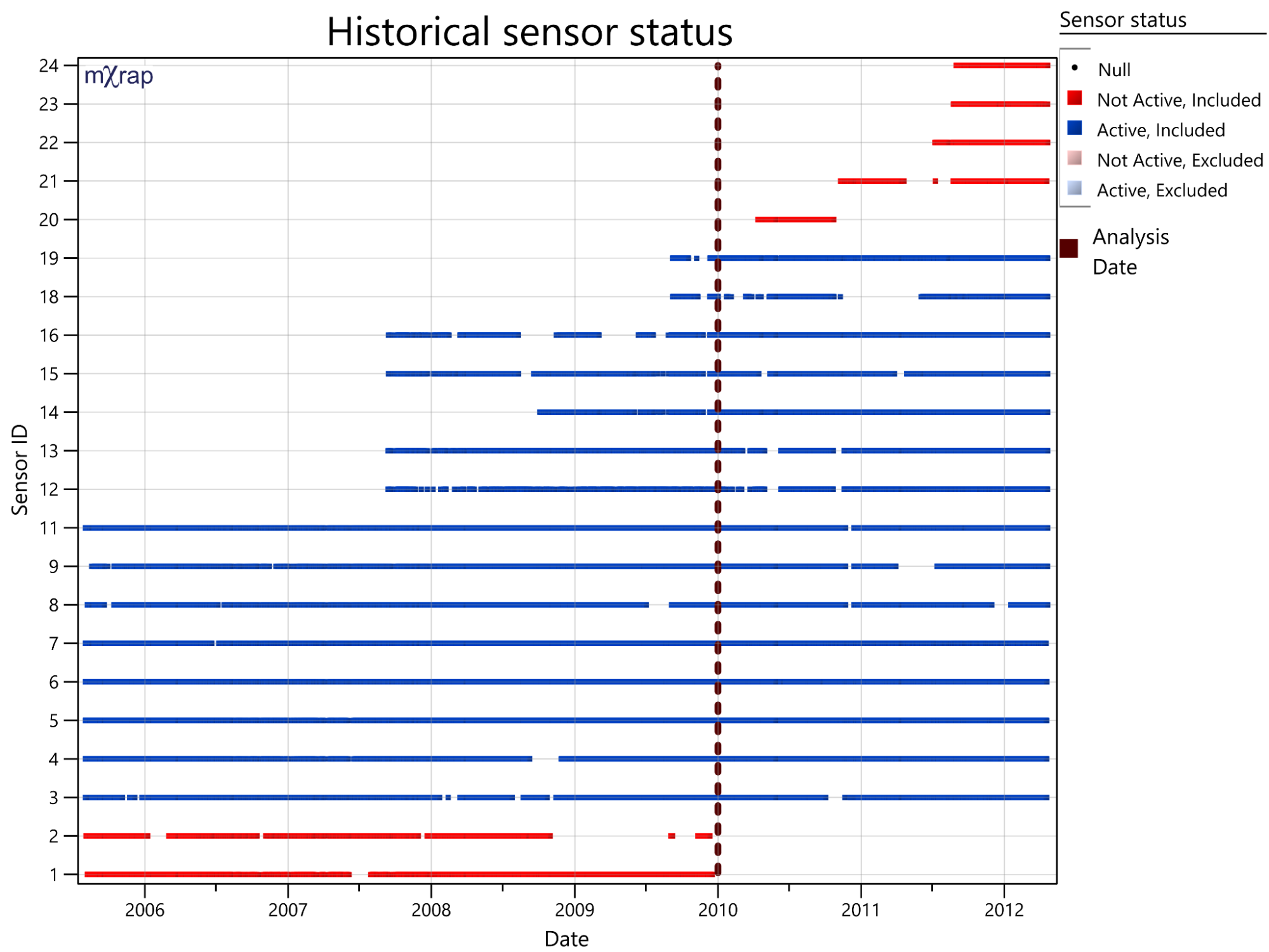
The second step is to establish your variables for your analysis in the analysis setup window. The main variable that needs to be set is the date (see figure) in the Control panel on the left. When you select a date, the sensors active on that day will be highlighted in blue in the Historical sensor status chart and the Current sensors table (see figures). Only the active sensors will be considered for the analysis.
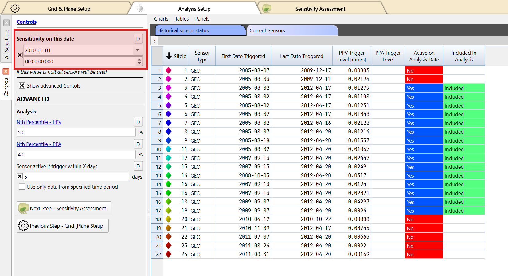
Additional tools in the window
If specific sensors need to be filtered, use the Sensor filters panel. If you tick the show advance Controls in the Controls panel, the Percentile value of the cumulative distribution that we use for each geophone to determine the trigger level can be modified as well as a buffer zone for sensor activity. These numbers are obtained by a specific calibration done by mXrap staff, please contact support if this calibration hasn’t been done for your mine.
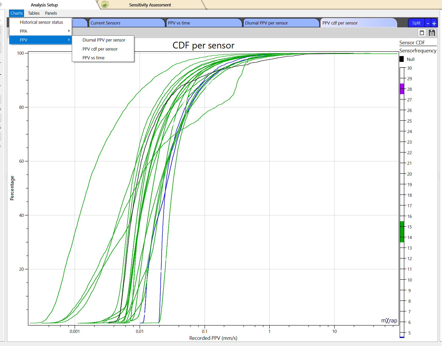
Additional charts can be also plotted to assess the distribution of PPA or PPV per sensor, so you can see if you have sensors that are more or less noisy, along with how the PPA/PPV changes during different times of the day or over the mine life.
Sensitivity assessment window
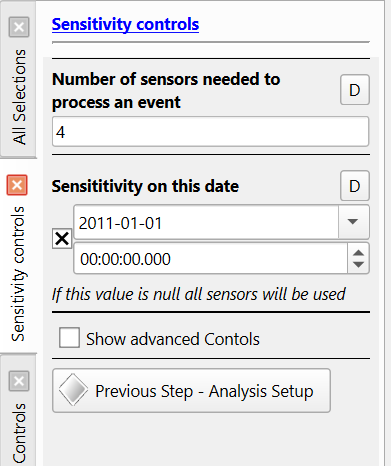
The number of sensors needed to process an event needs to be first imput in the Sensitivity controls panel. This number will have a significant impact on the analysis results. Most ESG/IMS systems have this number for processing. It is ideal to use the same number as the service provider.
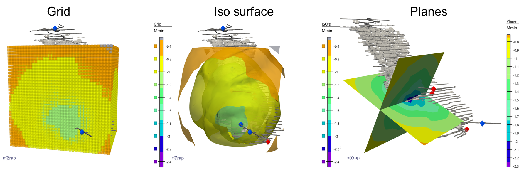
The main tool of this window is the 3D view which will display sensitivity across the mine based on the information set in the first 2 steps. There are 3 ways of displaying the sensitivity: grid points, Iso surface and plane (see figure). The marker style can also be changed to show the distance to Xth sensor (furthest sensor required to detect the event). The 3D view will also allow the display of the geometry model and sensors.
Use the slicing tool or override the marker transparency to help visualise the data.
Additional tools in the window
There are Sensitivity controls, Grid controls, Plane controls and Sensor filters panels to help quickly modify information set in the 2 previous steps.
There is a Grid Results table that can be exported to display the results in other softwares.