Moment tensors

• General Analysis
• Theory

tip

IMS and ESG sites should have moment tensors loaded in with the events table automatically.

Principal Axes

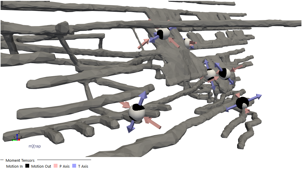
The principal axes are determined by diagonalising the full moment tensor. The orthogonal eigenvectors t, b, and p correspond to the maximum, intermediate, and minimum eigenvalues, respectively. The eigenvector t gives the tension axis, T, and the eigenvector p gives the pressure axis, P.

Note that, because the full moment tensor is diagonalised (rather than diagonalising only the double couple part), in moment tensors with high isotropic components it is possible that the P axis has a positive corresponding eigenvalue (for explosive sources), or that the T axis has a negative corresponding eigenvalue (for implosive sources). In 3D View plots of the principal axes, this will be visible as P and T axes arrows pointing in the same direction (either all towards the source location for implosive sources, or all away from the source location for explosive sources).

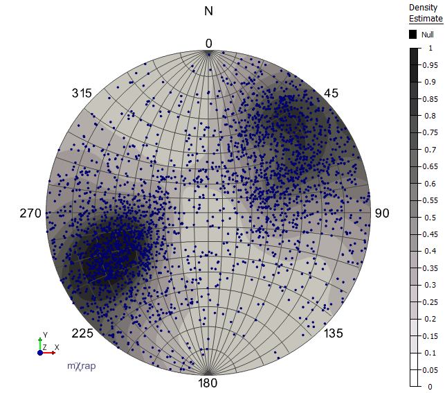
Principal Axes Density Plot

The principal axes density plot uses two distinct methods for visualising density estimates. The method used depends on the marker style chosen (in the "Show, and colour by" drop-down menu of the Density Estimate series). They can be broadly categorized as Density Estimation or Kernel Splattering, each of which is described further below.

Density Estimation

The density estimation methods work by counting the number of points within a certain distance of regularly spaced grid points (which cover the sphere, or one hemisphere for non-directed data such as the principal axes). This determines the density estimate at each grid point, after which contours can be created between neighbouring grid points where the density estimate crosses a particular value.

Kamb (1959)¹ described a method for contouring density diagrams of orientation data, based on the departure from a uniform distribution (e.g. regions with higher than expected density).

The mXrap implementation of density estimation is based upon the C program provided by Vollmer (1995)², and incorporates Vollmer's improvements upon Kamb's method:

• Parameterising the expected count: Parameterising the expected count for a random sample drawn from a uniform distribution (allowing one to lower the expected count reduces the smoothing of the orientation data, thus providing more localised density estimates). In the mXrap implementation, this parameter is exposed as the Sigma variable in the Density Estimation Controls section of the Principal Axes Density Plot 3D View Controls. It defaults to 3, the original value used by Kamb (1959).

• Using weighting methods for smoothing: As Vollmer (1995) explains:

  A simple tally of points within counting elements results in marginally satisfactory contours. Decreasing the grid spacing helps to bring out additional maxima by increasing the resolution of the contours, but tends to create jagged contours. The problem is that the density estimate at a point must be made over a finite area. In standard counting each data point within an element is assigned a weight, w, of 1, whereas a weight of zero is given to all points outside.

  The solution is to use weighting functions so that data points have a greater influence on grid points that are close to them, and progressively less influence on grid points further away from them. In the mXrap implementation the weighting function can be selected through the Select density estimation method table in the Density Estimation Controls section of the Principal Axes Density Plot 3D View Controls: Kamb (No Smoothing) selects the Kamb counting method with no weighting function applied, Kamb (Inverse Area Smoothing) selects the Kamb counting method with the inverse area weighting function applied (Vollmer 1995, Eq. 16), and so on.

• Estimating point density on the sphere: Estimating point density on the sphere (as opposed to estimating point density on, e.g. a stereonet projection). This is a natural extension for a program implementation, given that it is more computationally efficient (and straightforward to implement). The mXrap implementation also estimates point density on the sphere.

Kamb's method, no smoothing, sigma=3

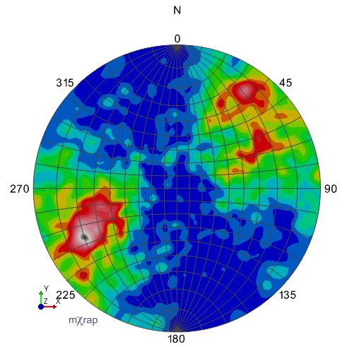Kamb's method, exponential smoothing, sigma=3 (default)

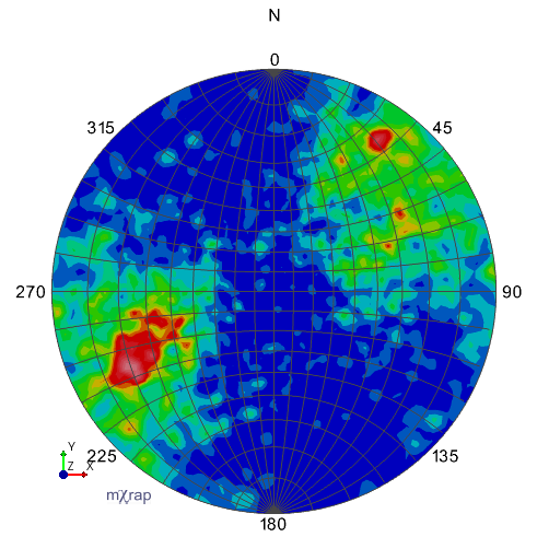Kamb's method, exponential smoothing, sigma=2

Kernel Splattering

The kernel splattering method estimates and plots density by counting data points within a specified distance of regularly spaced grid points. This method uses an icosphere to define grid points, ensuring each point is equidistant from its immediate neighbors. This approach contrasts with regular grids (such as those used by Vollmer, 1995) that are defined by equally spaced trend and plunge values, which create denser grid point concentrations near the sphere's poles.

For each combination of data point D and grid point G, with orientations defined by unit vectors d and g, the angle of separation is calculated as:

$\cos(\theta) = \mathbf{d} \cdot \mathbf{g}$

where $\mathbf{d} \cdot \mathbf{g}$ is the dot product of the unit vectors d and g.

The values from each data point D are "splattered" onto all grid points with an angle of separation less than or equal to $R_{max}$. These grid points are called the neighbours of D.

Since the principal axes are non-directional, data points are also splattered onto grid points at the opposite side of the sphere, using:

$\cos(\theta) = |\mathbf{d} \cdot \mathbf{g}|$

A kernel function $f$ is used to calculate how much the value of data point D should be splattered onto each neighbour grid point G, based on the angle of separation $\theta$, e.g. $kernel(D,G) = f(\arccos(|\mathbf{d} \cdot \mathbf{g}|)/R_{max})$.

The kernels are normalised by the sum of all kernel values calculated for a given data point and all of its neighbour grid points:

$\text{kernel}_{\text{normal}}(D,G) = \frac{\text{kernel}(D,G)}{\sum_{G} \text{kernel}(D,G)}$

This ensures that the sum of a data point's splattered value is equal to the data point's original value. For density estimation, this ensures that the expected density is not altered. Note that the weighting functions used with the modified Kamb methods described in the Density Estimation section ensure the same property (Vollmer, 1995).

The data point's values are then added to the neighbour grid points values based on the normalised kernel, with the end result being that:

$value(G) = \sum_{D} kernel_{normal}(D,G) \times value(D)$

The normalisation ensures that the sum of the values of all grid points equals the sum of the values of all data points.

The splattered count at each grid point can be normalised by the area of the sphere owned by one grid point. This provides a count that is affected by the total number of events, but is not affected by the number of grid points (determined by the number of icosphere refinements), nor the kernel function used, nor the maximum splatter distance $R_{max}$. This value is shown by the Kernel-Splattered Count marker styles in the Show, and colour by option of the Density Estimate series in the Principal Axes Density Plot.

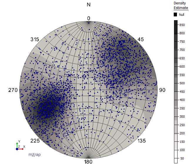
Kernel-Splattered Count: Colours indicate event density based on splattered event counts. The density estimate values will change based on the number of events being splattered, but will remain stable regardless of the icosphere grid density, kernel function, and maximum splatter distance.

The splattered count is also used to create the Kernel-Splattered Equi-probability Zones marker style. With this marker style, areas of the same colour contain the same number of (splattered) events. The lowest colour on the scale indicates the region with the least event density, and each successive colour on the scale indicates regions of increasing event density.

Kernel-Splattered Equi-probability Zones: The region defined by the darkest colour (0.9 to 1.0) has the same number of splattered events as the other coloured regions, but covers the least area (i.e. has the highest event density). The region covered by the lightest colour (0 to 0.1) has the lowest event density.

Decompositions

Standard Decomposition Formula

Moment tensor decompositions (as displayed in Picked Event Analysis, and as used to generate the radiation patterns on beach balls in the General Analysis and Large Event Analysis 3D Views) can be expressed as:

$\mathbf{M} = M_{\text{isotropic}} + M_{\text{DC}} + M_{\text{CLVD}}$

Theoretical Foundation

The decomposition is based on the formulae given by Vavryčuk (2015)³ in Section 3 (Standard moment tensor decomposition), and is equivalent to the comparable decomposition as described by Jost and Herrmann (1989)⁴.

Scalar Seismic Moment Calculation

For the scale factors $C_{\text{isotropic}}$, $C_{\text{DC}}$, $C_{\text{CLVD}}$, the formula for scalar seismic moment $M$ is:

$M = |M_{\text{ISO}}| + |M_{\text{CLVD}}| + M_{\text{DC}}$

Display and Configuration

These scale factors are displayed as percentage values in the user interface:

• % isotropic
• % deviatoric
• % DC
• % CLVD

These percentages can be viewed in the Events passing "Base Filter" table.

nota

Alternative decomposition methods can be selected through the Decomposition Methods control panel.

Hudson Plot

The Hudson plot is generated according to the original method given by Hudson et al. (1989)⁵. This plot does not change when alternate decomposition methods are selected (see above). Event densities are determined within grid cells formed by intersecting lines of equal k and T. For example, if the parameter Grid Cells for k,T is set to the default value of 20, then there are lines of equal k and T formed for the values -1, -0.9, -0.8, ..., 0.9, 1.0. Thus there will be a grid cell that contains all events with k in the range [-1, -0.9] and T in the range [-1, 0.9], and so on. The density of each grid cell is the number of events falling within that grid cell divided by the total number of events (passing the current filter).

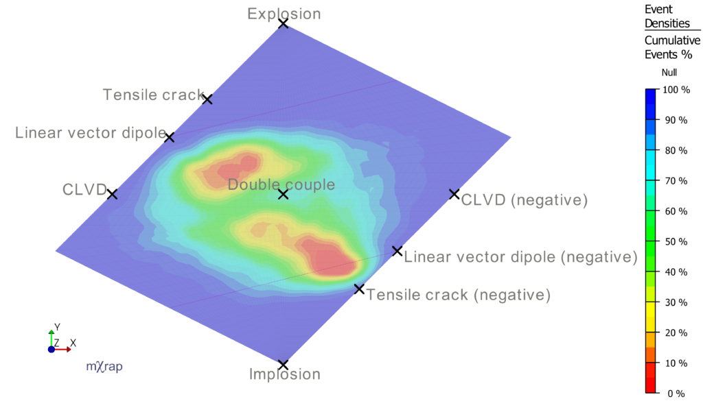
Diamond CLVD-ISO Plot

The Diamond CLVD-ISO plot is generated according to the selected decomposition method. By default this follows Jost and Herrmann (1989), but others can be selected through the Decomposition Methods control panel.

Moment Calculation Comparison Chart

This chart compares values for the seismic moment calculated from the moment tensor against the value for the seismic moment from the event database. If there is a very large (orders of magnitude) mismatch between these values (i.e. the dots are not grouped on the line of perfect agreement), it may indicate an error with moment tensor importing.

nota

You should contact to help determine whether there is an error and, if so, how to resolve it.

Moment Tensor Guide

Footnotes

1. Kamb, W.B. (1959). Ice petrofabric observations from Blue Glacier, Washington, in relation to theory and experiment. Journal of Geophysical Research, Vol. 64 (Issue 11), 1891-1909. doi: 10.1029/JZ064i011p01891 ↩

2. Vollmer, F.W. (1995). C program for automatic contouring of spherical orientation data using a modified Kamb method. Computers & Geosciences, Vol. 21 (Issue 1), 31-49. doi: 10.1016/0098-3004(94)00058-3 ↩

3. Vavryčuk, V. (2015). Moment tensor decompositions revisited. Journal of Seismology, 19:231-252. ↩

4. Jost, M.L., Herrmann, R.B. (1989). A Student's Guide to and Review of Moment Tensors. Seismological Research Letters, 60:37-57. ↩

5. Hudson, J. A., Pearce, R. G., and Rogers, R. M. (1989). Source type plot for inversion of the moment tensor. J. Geophys. Res., 94(B1), 765-774. doi: 10.1029/JB094iB01p00765 ↩