Grid Based Analysis
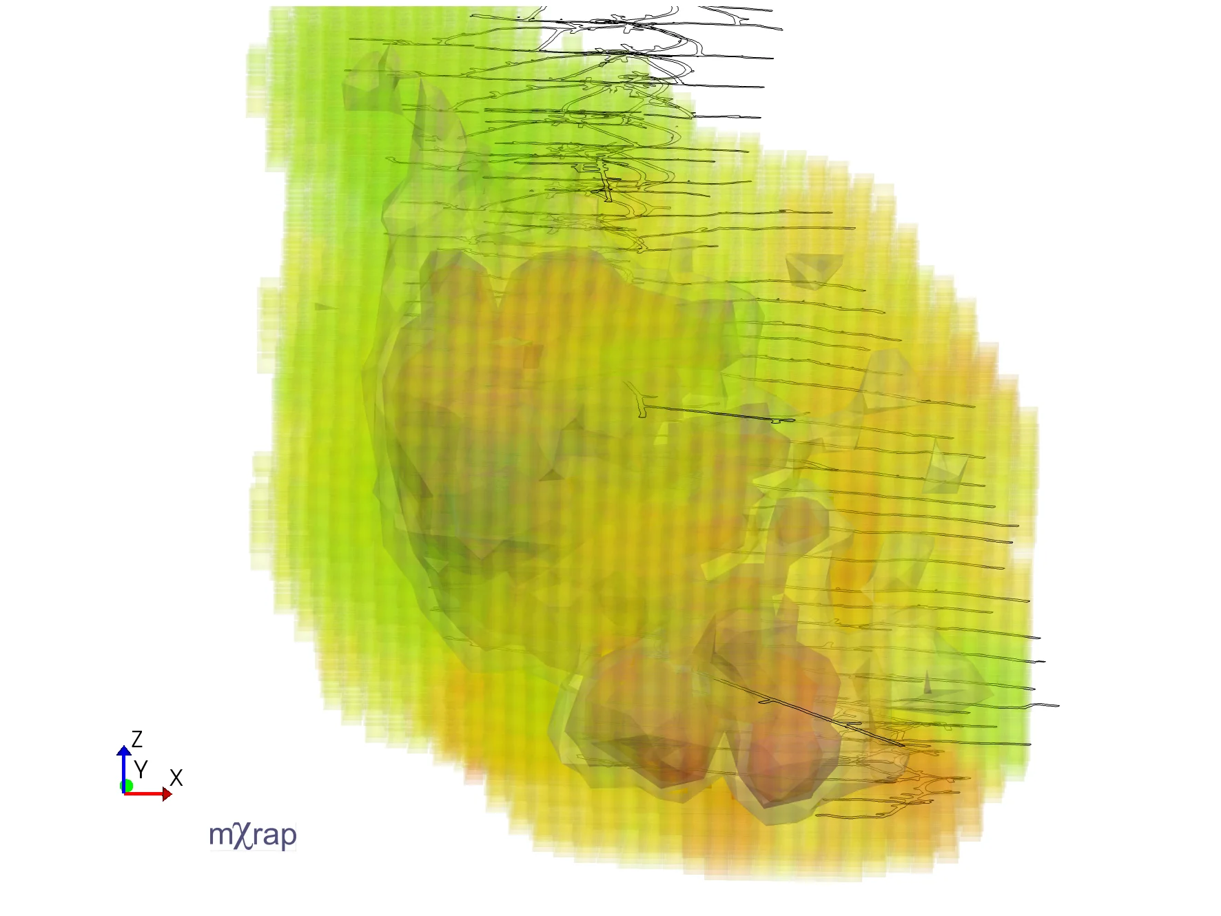
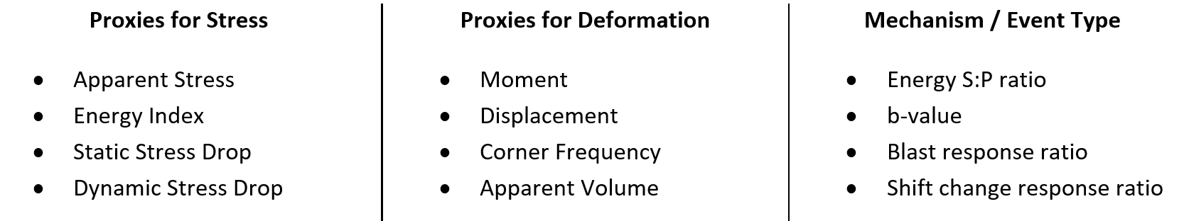
The Grid Based Analysis application can be used to evaluate the spatial distribution of various seismic parameters. There are a range of source parameter options available, and they can give indications to the rock mass behaviour. Some parameters can be considered as a proxy (stand-in) for rock mass stress, while other parameters can be a proxy for the amount of deformation. There are also parameters available that are associated with the rock mass mechanism or event type.
In grid-based analysis, a representative value of each seismic parameter is assigned to each grid point based on nearby events. This post summarises the calculation methods and control parameters used to assign each seismic parameter to the grid.
Parameters
Average versus cumulative parameters
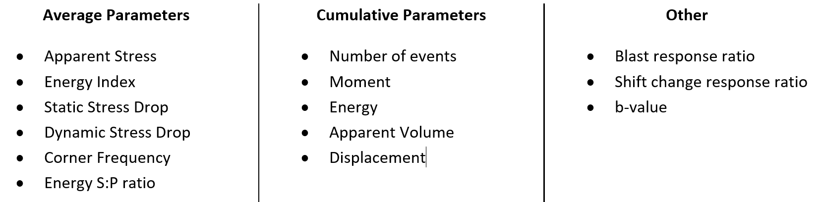
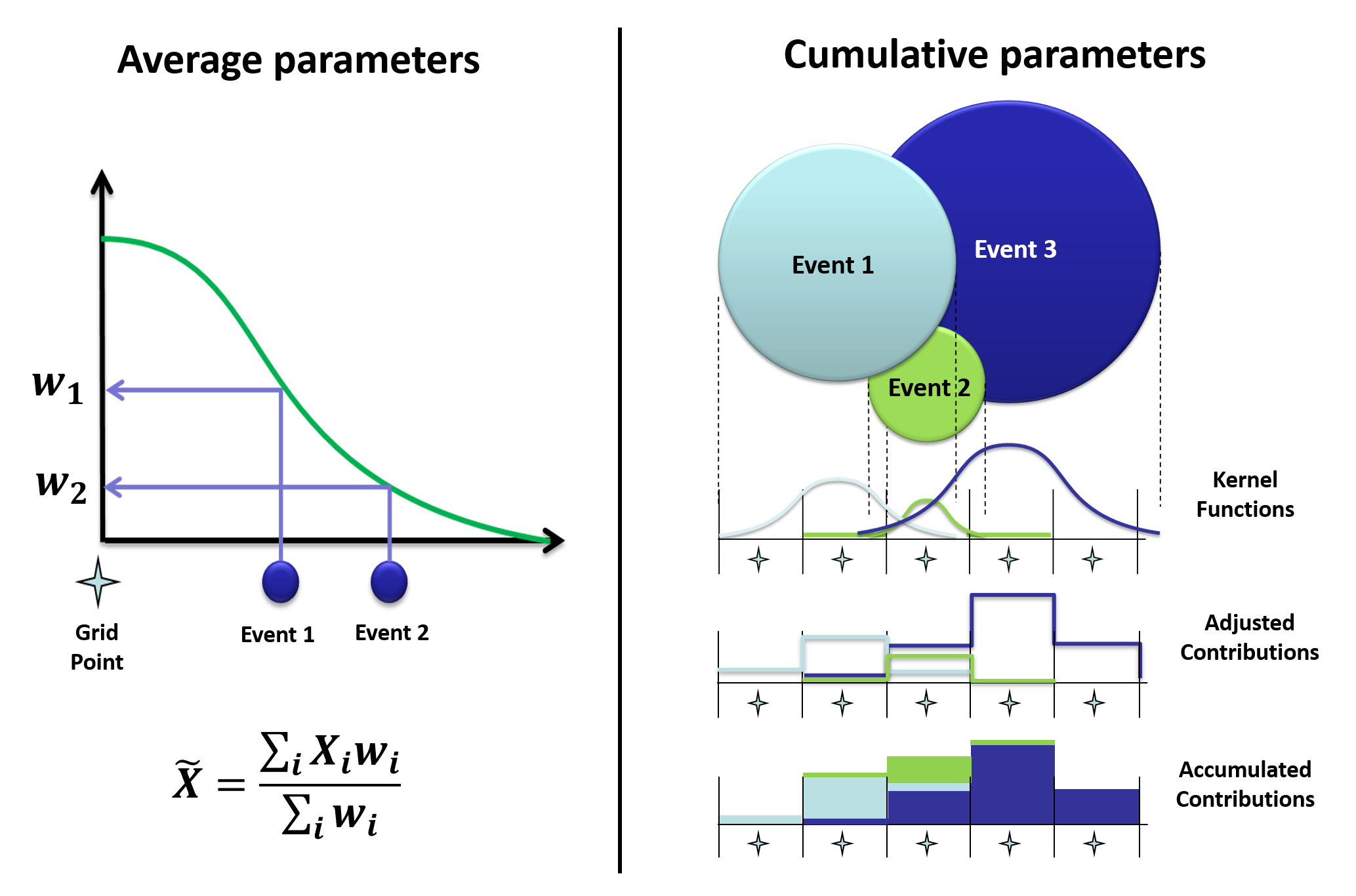
Most of the source parameters in the grid-based analysis app are what we call average or cumulative parameters. This is a distinction both in the nature of the parameter and the underlying calculation method. For some parameters, particularly those associated with rock mass deformation, it makes sense to find the cumulative effect of each event. Like moment for example, the salient information is how much deformation there has been in a certain area. For other parameters, generally related to stress (like energy index), the cumulative value doesn't really have much meaning. This is where we are interested in the average value instead. For parameters that scale exponentially, the average is calculated for log10(parameter).
The search radius
Grid-based analysis is fundamentally about associating nearby events with grid points. The event-grid association is made within a certain search radius, which is defined differently for average parameters and cumulative parameters.
For average parameters, a different search radius is used for each grid point, based on the event density nearby. There are three parameters to control the search radius around each grid point:
-
- Rmin. Minimum search radius. All events within this distance from the grid point are assigned, no matter how many there are. Default: 2 x Grid Spacing.
- Search N. The search radius is expanded until at least these many events are within range. Default: 50 events.
- Rmax. Maximum search radius. The search radius does not expand beyond this range, even if the Search N has not been reached. Default: 8 x Grid Spacing.
- Rmin. Minimum search radius. All events within this distance from the grid point are assigned, no matter how many there are. Default: 2 x Grid Spacing.
A density-based quality check is applied to all grid cells. At least 10 events must be found within a certain threshold distance of the grid point. The default distance is 90 (in native units). If there are less than 10 events within this range, no value is given to that grid point.
For cumulative parameters, rather than defining a search radius for each grid point, the search radius is different for each event, depending on the source size (source radius). No matter what the source radius is for an event, the search radius will not be set below 1.5 times the grid spacing, or above 200 m. The radius is converted to feet if that is the native spatial unit.
The kernel function
The search radius defines which events are associated with the grid but parameters are weighted depending on how close the event is to the grid point. The kernel function is what defines this distance weighting.
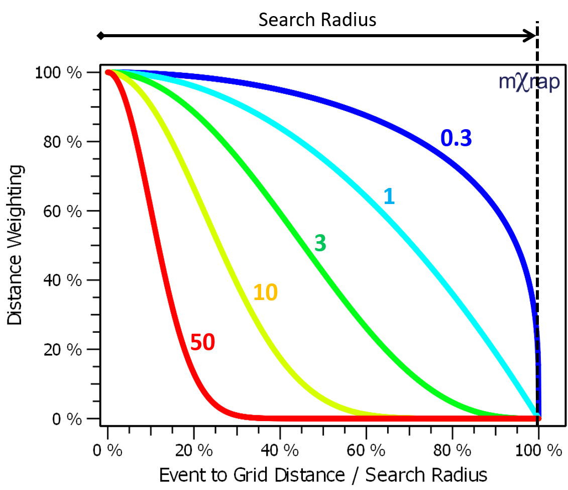
The kernel function order defines the shape of the kernel function. Various kernel functions are plotted on the right for kernel orders between 0.3 and 50. The default kernel function order is 3.
For average parameters, the inverse-distance weighted mean is calculated using the specified kernel function. For cumulative parameters, the kernel function controls how each event is distributed onto the grid cells. The contribution to each grid point is adjusted to ensure the cumulative parameters are conserved. In other words, if you compute the grid using 100 events or 1kJ of energy, the final result on the grid should also add up to 100 events or 1kJ.
Shift Change / Blast response ratio
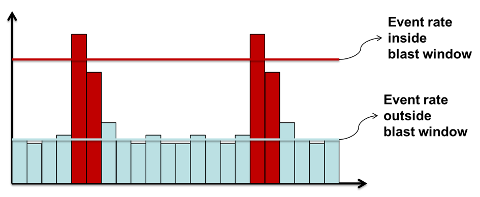
The response ratio for blasts and shift change is based on the event time of day. Blast and shift change periods are defined in General Setup Windows/Grid-based Analysis Settings. The response ratio is the activity rate inside the specified time-of-day periods divided by the activity rate outside those periods.
A high blast response ratio, for example, means there are a lot of events associated with blasting, and much less activity throughout the rest of the day. A blast response ratio of below one indicates the activity rate is higher during production periods, which is a sign of ore pass or other production noise dominating the dataset.
The search radius for calculating the response ratios are the same as the average parameters; a minimum number of events within a minimum and maximum radius. The difference is that there is no distance weighting applied, all events inside the search distance are treated the same.
b-value
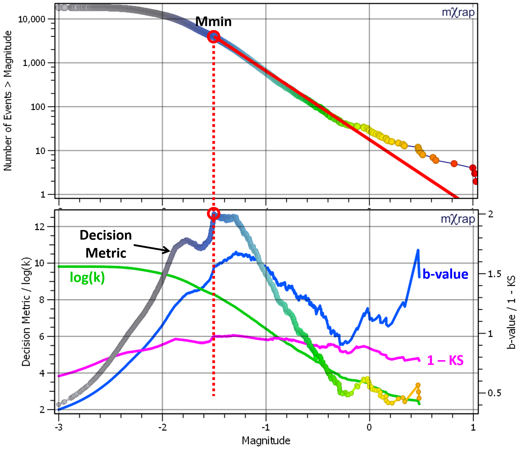
The event-grid association for the b-value calculations is the same as for the blast and shift change response ratios, i.e. not weighted by distance. A decision metric is used to find the Mmin (magnitude of completeness) for each grid point. Once the Mmin is known, the b-value can be calculated based on the average magnitude above Mmin.

The decision metric to find Mmin has three components:
-
- Log10(k). k is the number of events above Mmin. This is part of the decision metric so that as many events are found above Mmin as possible, and to push the solution away from the distribution tail, where there are few events and the other parameters are erratic.
- b. The b-value is part of the decision metric to avoid over-shooting the Mmin. Higher b-values are given more weight since underestimating Mmin would result in a lower b-value.
- 1 - KS. The KS value is a measure of the goodness of fit between the data and the Gutenberg-Richter model.
- Log10(k). k is the number of events above Mmin. This is part of the decision metric so that as many events are found above Mmin as possible, and to push the solution away from the distribution tail, where there are few events and the other parameters are erratic.
An example of the decision metric calculation is illustrated in the figure below, along with each of the three components. The metric is calculated for each event, as if it were the Mmin. To speed things up in the grid calculations, the metric is evaluated in bins, usually 0.1 magnitude units so you will generally only get Mmin to one decimal place in the results. The final Mmin is when the decision metric is at its maximum value.

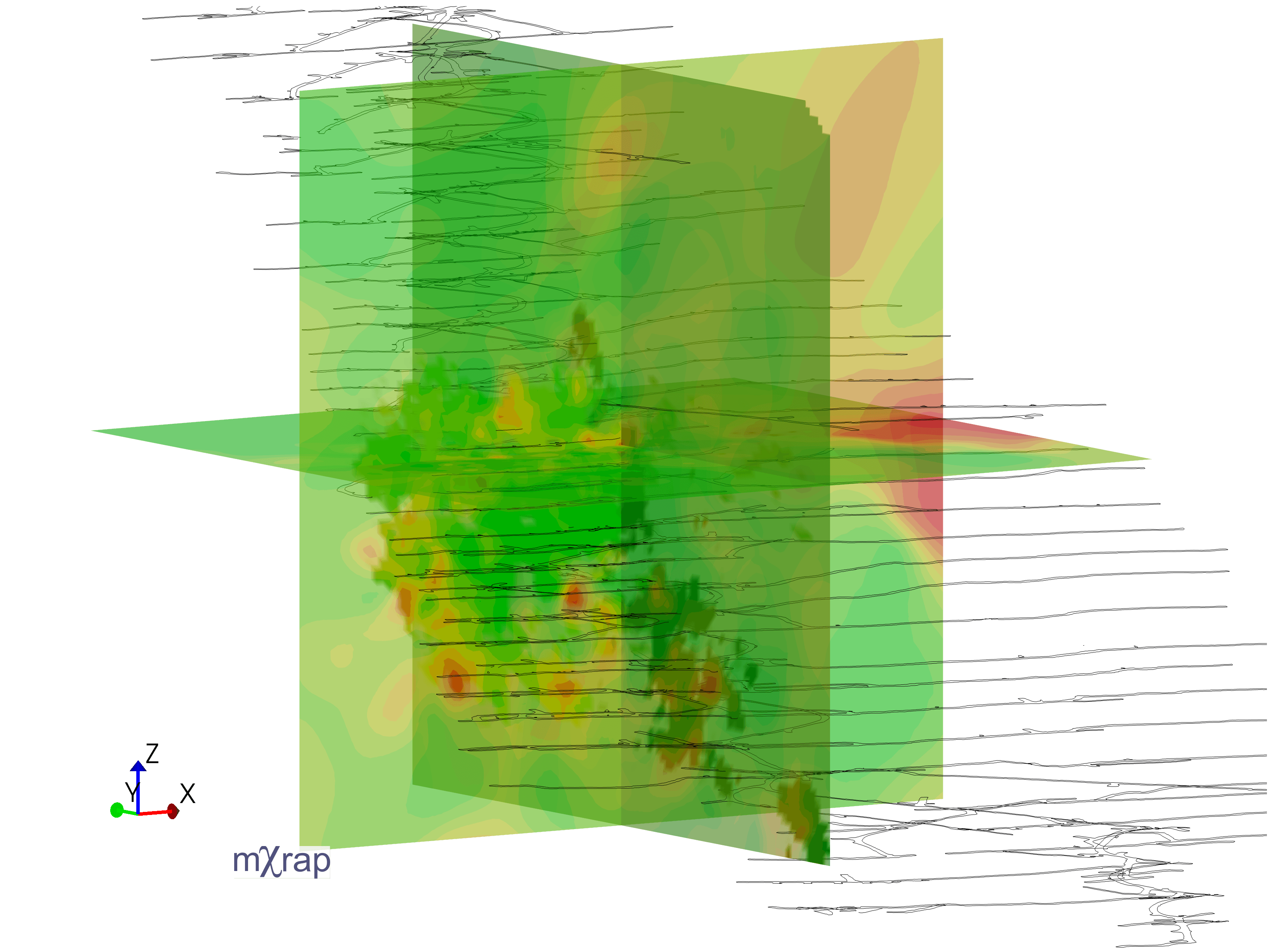
Plane-Based Analysis
The user can select a plane (defined in the plane editor window) and display cumulative or average parameters on that plane. Like the grid, the average and cumulative parameters are calculated differently. For the average parameters, the plane points are treated identically to the grid - the events around each point are found and the average parameter is calculated (the plane is essentially a 2D grid). The cumulative parameters are calculated on a 'splatter' basis; where events within a certain distance of the plane are projected onto the plane and their impact is distributed among the plane points within their source radius.
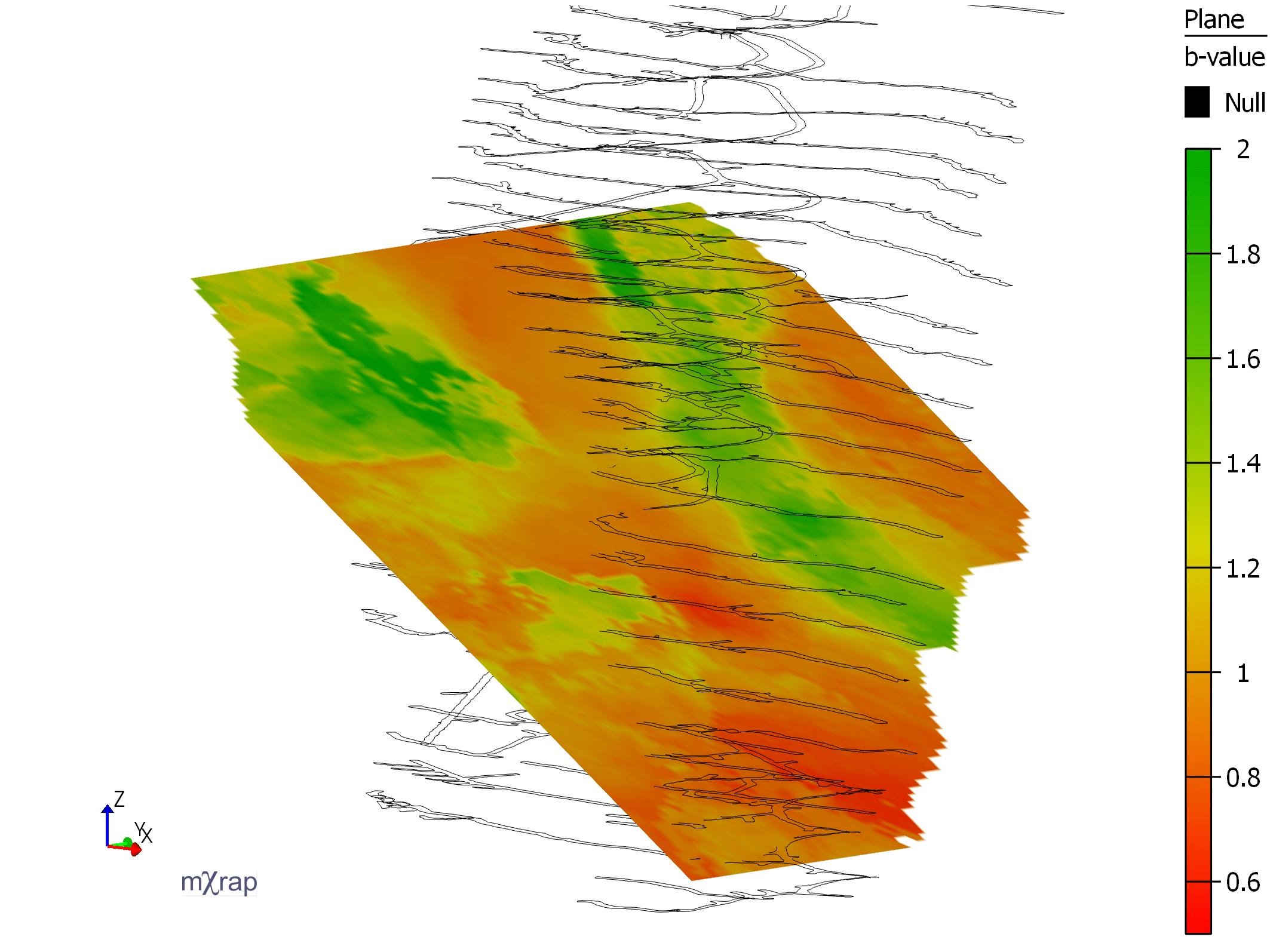
Plane based analysis can be used to try to evaluate the change in seismic parameters along a fault plane, or simply to view changes in parameters easily as a slice. The plane can be dynamically overridden, allowing the user to 'sweep' through their mine.
Several transparency options are available, including transparency based on a single value, based on the value of the parameter of interest or based on the number of events in the area (analysis quality).
Event Density Isos
This app is for the simple analysis of event density. You can use the basic date min and max range or the time-slicing function to see how event density changes over time.
Event density is computed based on a 3D grid. The contribution of each event on the grid is inversely proportional to distance. The maximum radius of influence of an event is a function of the source radius. Larger events have a larger zone of influence than small events. The total contribution of each event is readjusted to one. This ensures that the total event count based on density is the same as the actual event count.
The key parameter to display event density is the minimum density. This is expressed as the number of events in 10^6 m^3 volume (i.e. a 100 x 100 x 100 m cube). Areas with lower density than this value are not shown. Additional isosurfaces are displayed as a function of the minimum density to denote increasing density.
Updates
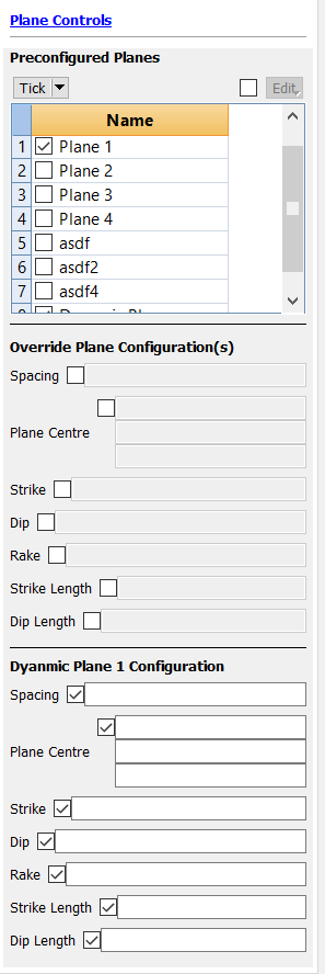
There are a number of updates to the Grid Based Analysis app. The first is the ability to use multiple planes for analysis instead of just a single plane.
You can also now choose up to two dynamically generated planes, instead of just the saved planes.
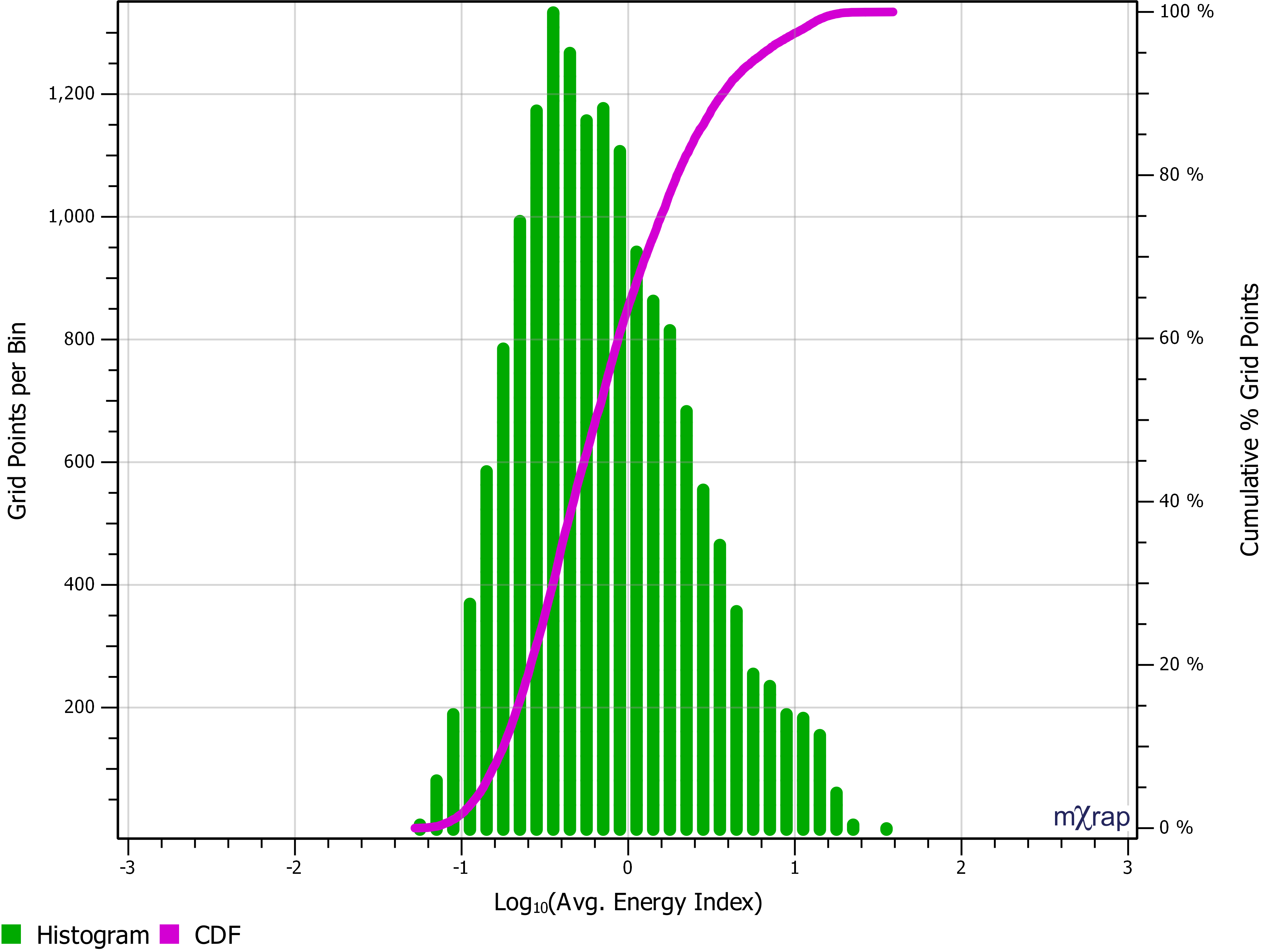
There is a new chart called 'grid results distribution' which gives both a histogram and cumulative distribution of the grid results so you can dig further into your results.
The last is a streamlining of the 'advanced' features. This makes it easier to compare different parameters in both the long and short term, using the grid and isosurfaces. Users can set a longer term and shorter term time period to identify areas of interest where seismicity in the short term differs from the longer term 'norm' for the mine. Using the transparency function on the grid can help to highlight these areas of interest.